Pre-implemented Modules - Part II
- “If you were plowing a field, which would you rather use: two strong oxen or 1024 chickens?”
This tutorial has two parts. In the first part, we showed how you can create pre-implemented modules tailored to fit your architecture. In this second part of the tutorial, we show how to assemble the PicoBlaze instances into a programmable overlay. To accomplish this, we will perform the following tasks:
1. Implementation Optimization: Use RapidWright and Vivado to get the best PicoBlaze implementations.
2. Building the Overlay: Replicate and stitch our pre-implemented PicoBlazes into an overlay.
1. Implementation Optimization
From Pre-implemented Modules - Part I, we finished by creating three pblocks to be used for our PicoBlaze implementation. Now that we know what our three pblock sizes are, we can use PerformanceExplorer, a tool provided with RapidWright, to help us explore implementation performance of each of these instances. The PerformanceExplorer is able to parallelize many different runs of place and route using different directives and also sweep clock uncertainty to explore the solution space. By leveraging Vivado and RapidWright’s PerformanceExplorer, we are able to capture the best implementation runs for reuse.
The RapidWright PerformanceExplorer can be run directly from the command line:
rapidwright PerformanceExplorer -h
which prints help and options detail:
==============================================================================
==                         DCP Performance Explorer                         ==
==============================================================================
This RapidWright program will place and route the same DCP in a variety of
ways with the goal of achieving higher performance in timing closure. This
tool will launch parallel jobs with the cross product of:
   < placer directives x router directives x clk uncertainty settings >

Option (* = required)                    Description
---------------------                    -----------
-?, -h                                   Print Help
-b <String: PBlock file, one set of
  ranges per line>
* -c <String: Name of clock to
  optimize>
-d [String: Run directory (jobs data     (default: <current directory>)
  location)]
* -i <String: Input DCP>
-m [String: Min clk uncertainty (ns)]    (default: -0.1)
-p [String: Comma separated list of      (default: Default, Explore)
  place_design -directives]
-q [Boolean: Sets attribute on pblock    (default: true)
  to contain routing]
-r [String: Comma separated list of      (default: Default, Explore)
  route_design -directives]
-s [String: Clk uncertainty step (ns)]   (default: 0.025)
* -t <String: Target clock period (ns)>
-u [String: Comma separated list of
  clk uncertainty values (ns)]
-x [String: Max clk uncertainty (ns)]    (default: 0.25)
-y [String: Specifies vivado path]       (default: vivado)
-z [Integer: Max number of concurrent    (default: 12)
  job when run locally]
To run PerformanceExplorer for our PicoBlaze design and three selected pblocks, we would run the following at the command line (where picoblaze_pblocks.txt the pblock file from Part I):
Danger
DO NOT USE THIS IN A TUTORIAL VIRTUAL MACHINE, it will crash the VM. PerformanceExplorer is best used with a compute cluster (such as LSF). It can be used on a single workstation, but, the number of parallel runs combined with their length can quickly add up to days of compute time.
# DON'T RUN THIS IN A TUTORIAL VIRTUAL MACHINE
rapidwright PerformanceExplorer -c clk -i picoblaze_synth.dcp -t 2.85 -b picoblaze_pblocks.txt
The PerformanceExplorer will then create a unique directory and launch a Vivado run for each unique job specification. There are four main parameters by which a job can be specified:
Placer Directive (
place_design -directiveoption)Router Directive (
route_design -directiveoption)Clock Uncertainty (applied before placement, then removed before routing)
PBlock (optional)
In our run of PerformanceExplorer above, we have the following set:
[Default, Explore]
[Default, Explore]
[-0.100, -0.075, -0.050, -0.025. 0.0, 0.025, 0.050, 0.075, 0.100, 0.125, 0.150, 0.175, 0.200, 0.225, 0.250]
[pblock0, pblock1, pblock2]
This yields a total of 2 x 2 x 15 x 3 = 180 runs. On a single workstation, this would take several hours depending on the number of parallel cores used (defaults to half the number of CPU cores, use -z option to specific core count). To avoid this lengthy step in the tutorial, we provide histograms of the results and best implementations here:
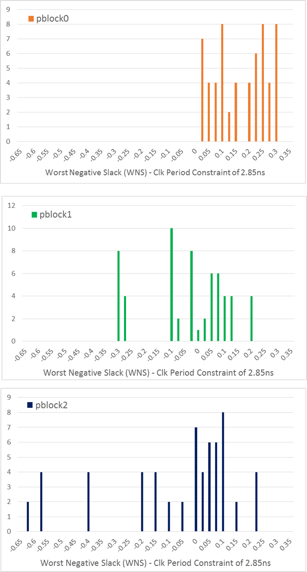
It seems Vivado was able to get the best performance from pblock0 which is the one with the floorplan that occurs most often. Although the histograms provide a view of what was achieved across 60 runs for each pblock, we really only care about the best results as those are what we move on with to the next step. For those curious, full performance results can be downloaded here: picoblaze_results.xlsx.
PBlock |
WNS (2.850ns period) |
Max Operating Freq. |
|---|---|---|
pblock0 |
0.300ns |
392MHz |
pblock1 |
0.178ns |
374MHz |
pblock2 |
0.207ns |
378MHz |
Download the best placed and routed implementations here: picoblaze_best.zip into your picoblaze directory then unzip the file:
unzip picoblaze_best.zip
2. Building the Overlay
Each PicoBlaze instance has a set of 4, 8-bit input ports {a,b,c,d} and 4, 8-bit output ports {w,x,y,z}. Our array of PicoBlaze instances will create columns on top of BRAM sites. The inter-module connectivity pattern for each column of PicoBlaze instances will follow this pattern:
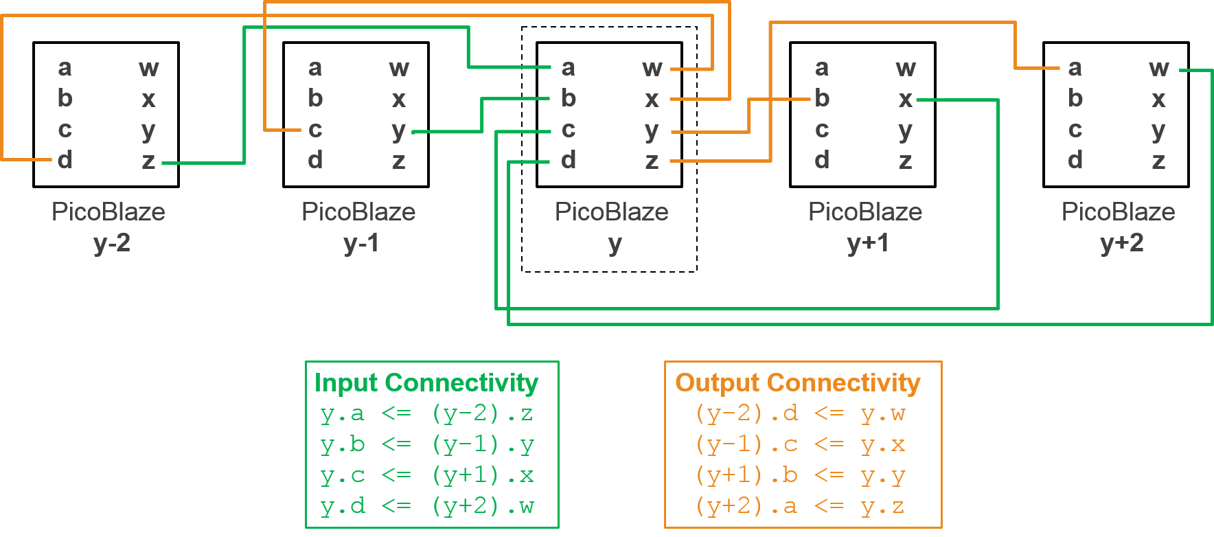
For each column, there will be one 8-bit top-level input that will drive any inputs that don’t have matching connecting instances. There will be one 8-top level output driven by the top PicoBlaze’s output z, all other outputs without matching connecting instances will be left unconnected.
RapidWright Java code to instantiate and place the three PicoBlaze pre-implemented modules and stitch them together is found in RapidWright/com/xilinx/rapidwright/examples/PicoBlazeArray.java. This can be run at the command line with the following command:
rapidwright PicoBlazeArray
Without any parameters, we get a simple usage message:
USAGE: <pblock dcp directory> <part> <output_dcp> [--no_hand_placer]
To run, we must provide the path to the directory where our pblock DCPs are located, the target device part name and an output DCP name:
rapidwright PicoBlazeArray `pwd` xcvu3p-ffvc1517-2-i picoblaze_array.dcp
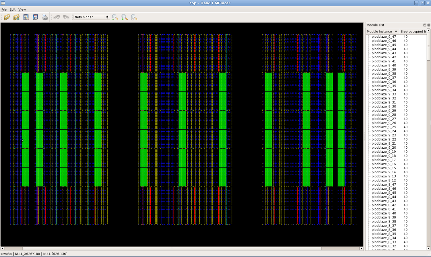
The program will read each of the pblock DCPs and stitch them together, printing out runtime numbers for each step. By default, the program will open the HandPlacer to enable the user to examine the placed PicoBlazes (you can skip the hand placer by adding --no_hand_placer as the last argument). Here is a screenshot of the tool:
You can zoom in/out using the scroll wheel of your mouse (or Ctrl + - to Zoom Out and Ctrl + = to Zoom In) and can move the pre-implemented PicoBlaze instances if you wish to change any of their placement. As you move the blocks, you’ll notice two things. First, the color of the block will change depending on its contextual location:
Green = Valid Placement
Orange = Valid Placement but overlapping
Red = Invalid Placement
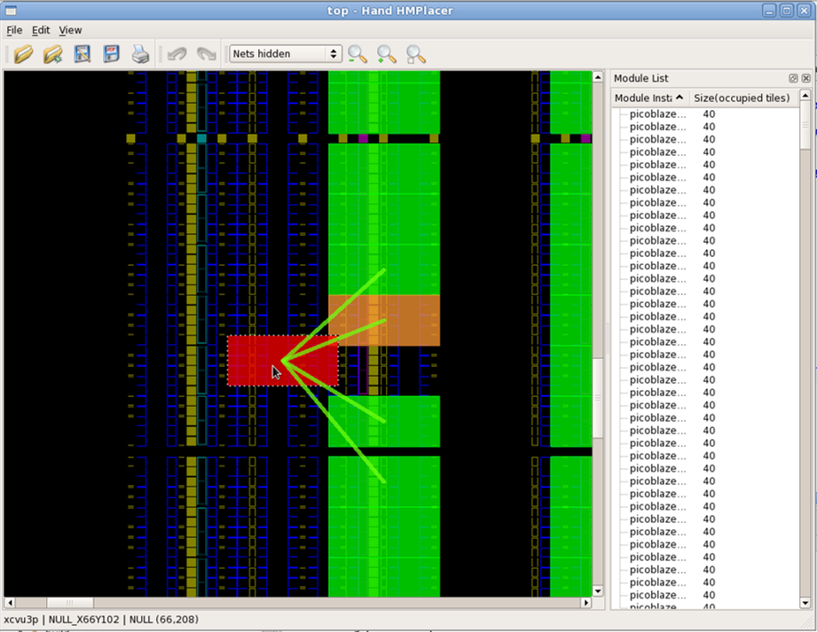
You’ll also notice colored lines that appear as you drag the blocks. These lines show high-level connectivity of the blocks to other blocks. The thicker the lines, the more tightly connected it is to its neighbors. If you choose to change the placement, its results will automatically be saved. Close the Hand Placer window, and the program will write out a placed and routed PicoBlaze array DCP.
Close any existing DCPs that are open in Vivado and open our new picoblaze_array.dcp:
close_design
open_checkpoint picoblaze_array.dcp
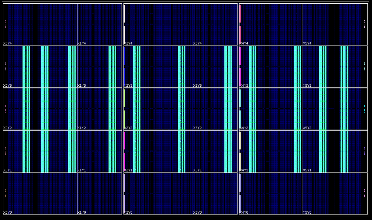
Once the design opens in Vivado, we find that RapidWright has “copied and pasted” our PicoBlaze 396 times in the center clock region rows of the VU3P as shown in the screenshot below:
To finalize the design, we simply need to update the clock tree, route the interconnections between PicoBlaze instances and check timing. This can be performed with the following Tcl commands:
update_clock_routing
route_design
report_timing_summary -delay_type min_max -report_unconstrained -check_timing_verbose -max_paths 10 -input_pins -routable_nets -name timing_1
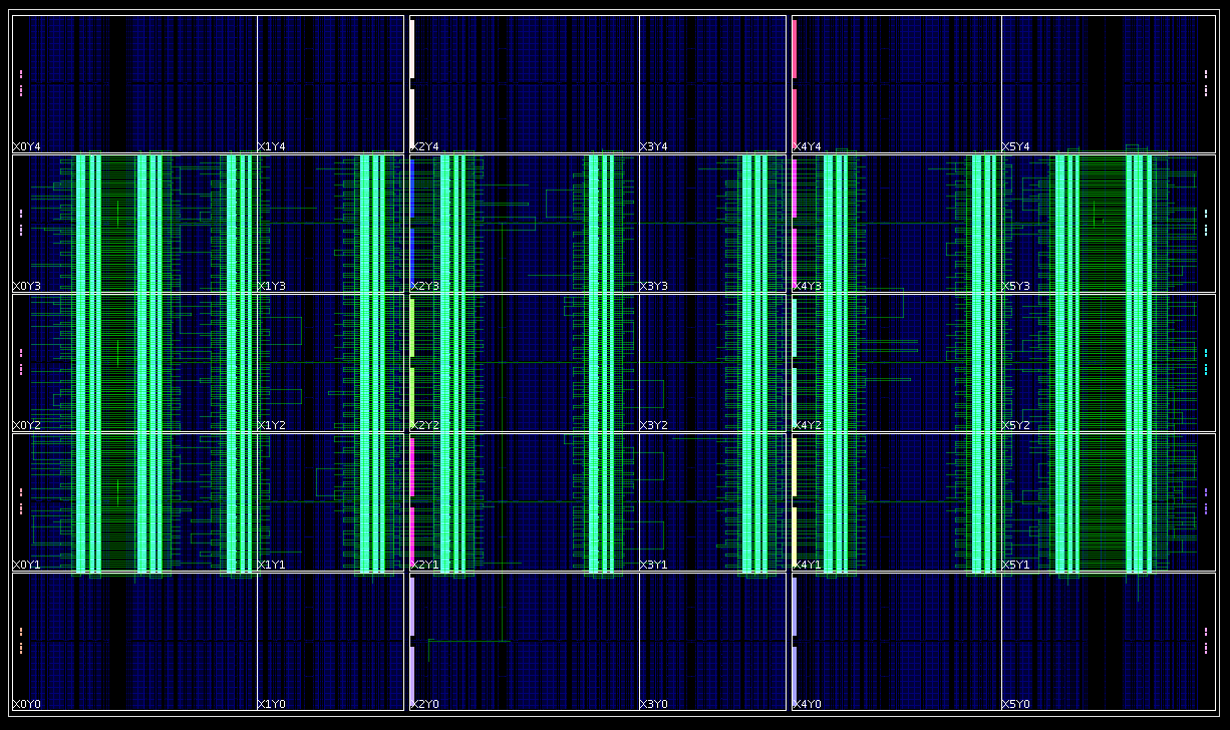
Once we are done, we should get a fully routed implementation that looks similar to this (or you can download our result here picoblaze_array_routed.dcp):
In our example, we had over 100ps of positive slack on the worst setup paths and meeting all hold requirements with at least 10ps of slack:
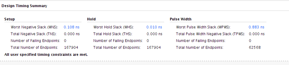
Although our clock period constraint is 2.85ns, we could run the array a bit higher at 365MHz. With some additional effort, we could increase the number of instances on the VU3P to 720 if we were to work around device edge cases, laguna tiles and one of the columns that wasn’t utilized due pattern overlap.
Conclusion
Although building an array of PicoBlaze microcontrollers probably won’t be used as the next architecture for deep learning acclerators or crypto miners, it has demonstrated how RapidWright and Vivado can be used together to achieve some interesting architectural structures in FPGA fabric. Specifically we have shown:
PBlock / Area Constraint Analysis - Getting the area constraint to the right footprint size
Tile Column Pattern Analysis - Picking the right patterns for maximum placement coverage
Performance Exploration - Using RapidWright and Vivado to find and harvest the best implementations
Overlay Construction - Using RapidWright to copy & paste implementations and stitch them together